301.01 - Parallel programming
Introduction
Historically, parallel "hardware" was developed in the early days of the mechanical computers (see: Charles Babbage, "The Analytical Engine"). The apparition of multi-core CPUs in the early 21st Century due to hitting the power wall led to an acceleration in the adoption of parallel computing.
- separating sequential computations into parallel sub-computations is often challenging if not impossible;
- ensuring correctness is hard due to new kinds of errors;
Speedup is the main reason for dealing with this extra complexity.
Parallelism and concurrency are related.
Parallelism uses parallel hardware to execute code faster. Main concerns are:
- division into sub-problems;
- optimal use of parallel hardware;
With concurrency, multiple executions may or may not execute at the same time. Main concerns:
- when can an execution start;
- how to exchange information between concurrent execution blocks;
- access to shared resources such as memory or shared files;
Parallelism relies on an algorithmic approach to problems rather than code organization. Parallelism manifests on various granularity levels:
-
bit-level parallelism led to the increase of "words" in CPUs from 4 bit to 8-bit, 16-bit, 32-bit and more recently 64-bit;
-
instruction-level parallelism led to executing multiple instructions at the same time. A program such as:
val b = a1 + a2;
val c = a3 + a4;
val d = c + b;
can execute the first two instructions at the same time, because they are independent. However, the third instruction can only be executed after the first two instructions have completed.
-
task-level parallelism executes separate instruction streams at the same time, on the same or on different data. This is often achieved through software support and it is the main focus of this course.
There are many classes of parallel hardware:
- multi-core processors;
- symmetric multiprocessors (SMPs) - multiple single or multi-core CPUs connected to common memory via a bus;
- graphics-processing units (GPUs) - specialized co-processors;
- field-programmable gate arrays - general-purpose co-processors that can be rewired for a specific task, programmable with hardware-description languages;
- computer clusters - groups of computers connected via network and who do not have a shared memory;
Parallelism on the JVM
Assumptions:
- we are running the code on a multi-core or multi-processor system with shared memory;
- the code runs on a JVM;
Operating system is software that manages the hardware and software resources and schedules program execution.
Process is an instance of a program executing inside an operating system. Processes are the most coarse grained units of concurrency on a shared memory OS. Processes are multiplexed by the CPU using time slices. This is called multitasking. Processes have isolated memory spaces.
Each process can contain multiple concurrency units called threads. Threads share the same memory space. Each thread has a program counter and a program stack.
Each JVM program starts a main thread. On the JVM, in order to start a new execution thread we must:
- define a subclass of Thread;
- instantiate a new thread object;
- call start on the thread object;
class HelloThread extends Thread {
  override def run() {
    println("Hello world!");
  }
}

val t = new HelloThread

t.start()
t.join()
The memory model is a set of rules that governs how threads interact when accessing shared memory. For instance, when thread T1 writes a value into shared memory, what value does thread T2 see and when does it see it? There are two core rules of the memory model:
- two threads writing to different memory locations don't need synchronization;
- a thread X that calls join on a thread Y is assured to see all the writes of thread Y after the join returns;
Running computations in parallel
The most simple way of describing parallelism is the following:
parallel(e1, e2)e1 and e2 are two expressions that must be evaluated in parallel.
Take for instance the calculation of p-norm. A 2-norm is used to calculate the length of a vector:
$$ (a_1^2 + a_2^2)^{1/2}$$
In a p-dimensional space, the p-norm of a vector:
$$(a_1, a_2, ... a_n) $$
is:
$$ (\sum_{i=1}^n |a_i|^p))^{1/p}$$
Sequential solution
Subproblem: computing the sum of powers of an array segment. Given:
- an integer array a representing our vector
- a positive double floating point number p
- two valid indices: s and t in the vector
we must compute:
$$ (\sum_{i=s}^{t-1} |a_i|^p))$$
with
$$|a_i|^p$$
rounded down to an integer.
Writing this sequentially:
def sumSegment(a: Array[Int], p: Double, s: Int, t:Int): Int = {
  var i = s;
  var sum: Int = 0;
  while (i < t) {
    sum = sum + power(a[i], p)
    i = i+1
  }
  sum
}

def power(x: Int, p: Double): Int = math.exp(p * math.log(abs(x))).toInt
math.exp returns Euler's number: e raised to the power of a double value.
Once we have sumSegment we can calculate the p-norm as:
def pNorm(a: Array[Int], p: Double): Int
       = power(sumSegment(a, p, 0, a.length), 1/p)
Parallel solution
Notice that:
$$ (\sum_{i=0}^{n-1} |ai|^p)) = (\sum{i=0}^{m-1} |ai|^p + \sum{i=m}^{n-1} |a_i|^p)$$
For efficiency, we choose m to be somewhere in the middle of the vector:
def pNormTwoPart(a: Array[Int], p: Double): Int = {
  val m = a.length / 2
  val (sum1, sum2) = parallel(sumSegment(a, p, 0, m),
                      sumSegment(a, p, m, a.length))
  power(sum1+sum2, 1/p)
}
The parallel combinator will cause the execution of the two sumSegments to be run in parallel.
A generic recursive parallel algorithm:
def pNormRec(a: Array[Int], p: Double): Int =
        power(segmentRec(a, p, 0, a.length), 1/p))

// like sumSegment, but parallel
def segmentRec(a: Array[Int], p: Double, s: Int, t: Int): Int = {
  if (t-s < threshold) {
    sumSegment(a, p, s, t)  // small segment, do it sequentially
  }
  else {
    val m = s + (t-s)/2
    val (sum1, sum2) = parallel(segmentRec(a, p, s, m),
                                segmentRec(a, p, m, t))
    sum1 + sum2
  }
}
The signature of parallel is:
def parallel[A, B](taskA: => A, taskB: => B): (A, B) = { ..... }- returns the same values as given
- benefit: parallel(a, b) can be faster than (a, b)
- input arguments by name ( => A and => B )
Monte Carlo Method to Estimate Pi
This is an algorithm for estimating the value of Pi. Take a circle of radius 1 and a square that boxes the circle around. Alternatively, we can use just a quarter of the circle.
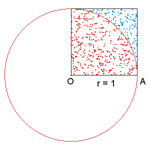
The ratio between the area of the square and the circle segment is:
$$ \lambda = \frac{(\frac{(\pi 1^2)}{4})}{1^2} = \frac{\pi}{4}$$
In order to estimate this ratio, we can randomly sample points within the square and calculate how many of them fall inside the circle. We then multiply the estimated ratio by 4 in order to obtain the estimation of Pi.
Sequential code to implement the Monte Carlo method
import scala.util.Random
def mcCount(iter: Int): Int = {
  val randomX = new Random
  val randomY = new Random
  var hits = 0
  for (i <- 0 until iter) {
    val x = randomX.nextDouble  // in [0, 1)
    val y = randomY.nextDouble  // in [0, 1)
    if ((x*x + y*y) < 1) {
      hits = hits + 1
    }
  }
  hits
}

def monteCarloPiSeq(iter: Int): Double = 4.0 * mcCount(iter) / iter
Parallel code to implement the Monte Carlo method (Four-way)
def monteCarloPiPar(iter: Int): Double = {
  val ((count1, count2), (count3, count4)) = parallel(
      parallel(mcCount(iter/4), mcCount(iter/4)),
      parallel(mcCount(iter/4), mcCount(iter-3*(iter/4))))
  4.0 * (count1 + count2 + count3 + count4) / iter
}
First-class tasks
A more flexible construct to describe parallel computations. Instead of using:
val (v1, v2) = parallel(e1, e2)we can use the task construct as follows:
val t1 = task(e1)
val t2 = task(e2)
val v1 = t1.join
val v2 = t2.join
t = task(e) will start the computation of e in the background.
- t is a task that computes the value of e
- current computation continues in parallel with t
- to obtain the value of e use t.join
- t.join blocks until the computation of e completes
- subsequent t.join calls immediately return the same result
A minimal interface for task looks like this:
def task(c: => A): Task[A]

trait Task[A] {
  def join: A
}
task and join establish maps between computations and tasks. In terms of the computed value, the following equation holds: task(e).join = e. We can ommit writing .join if we also define an implicit conversion:
implicit def getJoin[T](x: Task[T]): T = x.joinWe can now rewrite the four-way parallel p-norm:
val ((part1, part2), (part3, part4)) = parallel(
    parallel(sumSegment(a, p, 0, mid1),
             sumSegment(a, p, mid1, mid2)),
    parallel(sumSegment(a, p, mid2, mid3),
             sumSegment(a, p, mid3, a.length))
 )
power (part1 + part2 + part3 + part4, 1/p)
as follows:
val t1 = task {sumSegment(a, p, 0, mid1)}
val t2 = task {sumSegment(a, p, mid1, mid2)}
val t3 = task {sumSegment(a, p, mid2, mid3)}
val t4 = task {sumSegment(a, p, mid3, a.length)}

power (t1 + t2 + t3 + t4, 1/p)
Notice that because of the default declaration, reading the value of t1 will essentially invoke t1.join.
Assuming we have the definition for task, how can we rewrite the *parallel construction using it?
def parallel[A, B](cA: => A, cB: => b): (A, B) = {
  val tb: Task[B] = task {cB}  // tb execution spawned in parallel
  val ta: A = cA               // ta execution occurs in the "main" thread
  (ta, tb.join)                // tb.join blocks until the tb computation is finished
}
How fast are parallel programs?
Performance of parallel programs can be estimated using:
- empirical measurements;
- asymptotic analysis;
Asymptotic analysis is important to understand how algorithms scale when:
- inputs get larger;
- we have more hardware parallelism available;
We examine worst-case (not average) bounds.
For instance: the time bound on the sequential execution of the sumSegment function is: O(t-s), where t and s are the segment bounds. The time bound on the parallel execution of the sumRec function is: O(log(t-s)) due to the parallelism.
Work and depth
The conclusions above assumed an infinite number of parallel resources. When doing the asymptotic analysis of parallel algorithms, we use two measures:
- the work W(e) - the number of steps for the sequential execution of the algorithm
- the depth D(e) - the number of steps if we had unbounded (infinite) parallelism
Benchmarking parallel programs
Measuring performance usually leads to variable measurement results. In order to analyse the performance results we must:
- repeat the measurements multiple times;
- do a statistical analysis of the result (mean and variance);
- eliminate outliers;
- ensure a steady state when starting the program (warm-up);
- preventing anomalies (GC, JIT compiling, aggressive optimization, etc);
ScalaMeter is a benchmarking and performance regression testing tool on the JVM. Using ScalaMeter is done by adding its library to the sbt project:
libraryDependencies += "com.storm-enroute" %% "scalameter-core" %% "0.6"Then, in the testing code we would use the framework as follows:
import org.scalameter._

val time = measure {
  (0 until 1000000).toArray
}

println(s"Array initialization time: $time ms")
Running this program multiple times, we notice a wide range of outputs. This is because of the way that the JVM warms up:
- first, the program is interpreted;
- then, parts of the program are compiled into machine code (JIT);
- later, additional dynamic optimizations are applied;
- eventually, the program reaches a steady state;
What we want to measure is the steady state performance. With ScalaMeter we can do that:
import org.scalameter._

val time = withWarmer(new Warmer.Default) measure {
  (0 until 1000000).toArray
}

println(s"Array initialization time: $time ms")
A configuration clause can be used to tweak the parameters of the Warmer:
val time = config(
    Key.exec.minWarmupRuns -> 20,
    Key.exec.maxWarmupRuns -> 60,
    Key.verbose -> true
    ) withWarmer(new Warmer.Default) measure {
        (0 until 1000000).toArray
      }
ScalaMeter can measure more than just running time:
- IgnoringGC measures the running time without GC pauses;
- OutlierElimination measure removes statistical outliers from the measurement;
- MemoryFootPrint measures memory footprint of an object;
- Garbage collection cycles measures the total number of GC pauses during the execution of the benchmark;
- Newer ScalaMeter versions can also measure method invocation counts and primitive value boxing counts;
withMeasurer(new Mesurer.MemoryFootPrint) measure {
  (0 until 1000000).toArray
}